Motivation#

Anomaly detection is a case of binary classification. As such, we want to assign each data point a label 0 (normal) and 1 (anomalous). To measure the effectiveness of a detection method, we can calculate the following performance metrics:

Recall(RC): How much of anomalies is detected?
Precision (PR): How many predictions (for anomalies) concern real anomalies?
F1: The harmonic mean of recall and precision, which punishes a large spread.
Segments (SEG): How many anomaly segments are detected?

For time series data, i.e., a series of observations, we define an anomaly as a subsequence within. Naturally, this opens the possibility to two different approaches of calculation:

point-based: the prediction for each data point is compared to the corresponding label
range-based: a sequence predictions for an anomaly segment are compared against a sequence of labels (i.e., an anomaly)

In a point-based approach, we can categorize the predictions as follows:

true positives (TP): Number of label predictions that are correctly identified as anomalous
false positive (FP): Number of labels predictions that are wrongly classified as anomalous
true negatives (TN): Number of label predictions that are correctly identified as normal
false negatives (FN): Number of label predictions that are wrongly classified as normal

With this in mind, we would calculate the aforementioned performance metrics as follows:

\begin{align*} \mathrm{RC}^{\mathrm{P}}(\tilde{\mathbf{y}}, \mathbf{y}) & \triangleq \frac{\mathrm{TP}}{\mathrm{TP} + \mathrm{FN}} \\ \mathrm{PR}^{\mathrm{P}}(\tilde{\mathbf{y}}, \mathbf{y}) & \triangleq \frac{\mathrm{TP}}{\mathrm{TP} + \mathrm{FP}} \\ \mathrm{F1}^{\mathrm{P}}(\tilde{\mathbf{y}}, \mathbf{y}) & \triangleq 2 \frac{\mathrm{PR}^{\mathrm{P}} \cdot \mathrm{RC}^{\mathrm{P}}}{\mathrm{PR}^{\mathrm{P}} + \mathrm{RC}^{\mathrm{P}}} = \frac{2 \mathrm{TP}}{2\mathrm{TP} + \mathrm{FP} + \mathrm{FN}}\\ \mathrm{SEG}^{\mathrm{P}}(\tilde{\mathbf{y}}, \mathbf{y}) & \triangleq \sum_{\mathbf{A}_i \in \mathcal{A}} \mathbb{1}( \sum_{\mathbf{P}_j \in \mathcal{P}} |\mathbf{P}_j \cap \mathbf{A}_i| > 0) \end{align*}

where $\mathbf{y}$ are the labels and $\tilde{\mathbf{y}}$ the predictions.

A common variation to the point-wise approach was proposed by Xu et al. called point-adjust (PA). The idea of point-adjust is to mixture of a point- and range-based approach: An anomaly segment $A_i$ counts as detected if there is at least one correct prediction in the segment. This is achieved by adjusting the predictions $\tilde{\mathbf{y}}$ using the labels $\mathbf{y}$ as follows:

\[\begin{split}\tilde{y}^{\mathrm{PA}}_t = \begin{cases} 1, & \text{if $\tilde{y}_t = 1$ or $\mathbf{x}_t \in \mathbf{A}_i$ and $\underset{\mathbf{x}_{t'} \in \mathbf{A}_i}{\exists} \tilde{y}_{t'} = 1$} \\ 0, & \text{otherwise.} \\ \end{cases}\end{split}\]

The following example illustrates the changes that are made to the predictions $\tilde{\mathbf{y}}$ to obtain the adjusted predictions $\tilde{\mathbf{y}}^\mathrm{PA}$ (the changed positions are underlined):

\begin{align*} \text{labels} \; \mathbf{y}: & [\;0\;0\;1\;1\;1\;0\;0\;1\;1\;0] \\ \\ \text{predictions} \; \tilde{\mathbf{y}}: & [\;1\;0\;0\;0\;1\;1\;0\;0\;0\;0] \\ \text{adjusted} \; \tilde{\mathbf{y}}^\mathrm{PA}: & [\;1\;0\;\underline{1}\;\underline{1}\;1\;1\;0\;0\;0\;0] \\ \end{align*}

Afterward, we can calculate the recall, precision, f1, and segment score in the same way as before.

There are several problems with this approach. Mainly, that it overestimates the performance and that a higher f1 score does not necessarily constitute in a better detection method. For example, a detection method which only detects each anomaly segment by a single point is scored the same as a method which correctly detects the full segment (before the adjustment). For a more detailed discussion see Kim et al..

Range-based approaches compare a predicted anomaly segment to a real anomaly segment. Thus, it is possible that a prediction $P_j$ partially overlaps with an anomaly A_i. It can be partially a TP and partially a FP. How eTaPR (enhanced time-aware precision and recall) proposed by Hwang et al. handles this problem we will discussed in the next section.

eTaPR#

The motivation behind the eTaPR is that it is enough for a detection method to partially detect an anomaly segment, as along as an human expert can find the anomaly around this prediction. The following illustration (a recreation from the paper) highlights the four cases which are considered by eTaPR:

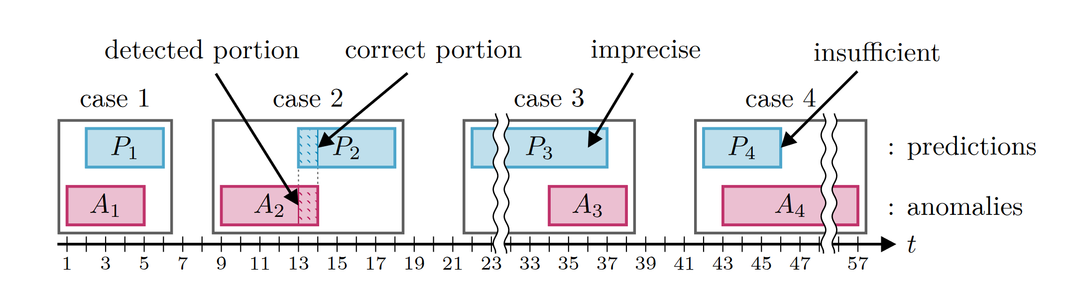
A successful detection: A human expert can likely find the anomaly $A_1$ based on the prediction $P_1$.
A failed detection: Only a small portion of the prediction $P_2$ overlaps with the anomaly $A_2$.
A failed detection: Most of the prediction $P_3$ lies in the range of non-anomalous behavior (prediction starts too early). A human expert will likely regard the prediction $P_3$ as incorrect or a false alarm. The prediction $P_3$ is too imprecise and the anomaly $A_3$ is likely to be missed.
A failed prediction: The prediction $P_4$ mostly overlaps with the anomaly $A_4$, but covers only a small portion of the actual anomaly segment. Thus, a human expert is likely to dismiss the prediction $P_4$ as incorrect because the full extend of the anomaly remains hidden. The prediction P_4 contains insufficient information about the anomaly.

Note that for case 4, we could still mark the anomaly as detected, if there were more predictions which overlap with the anomaly $A_4$. Specifically, the handling of the cases 3 and 4 is what sets eTaPR apart from other scoring methods.

In the next section, we will focus on the inner workings and how to calculate the eTa metrics. The basis are two subsets: a set of detected anomalies $\mathcal{A}^D \subseteq \mathcal{A}$ which is a subset of all anomalies and a set of correct predictions $\mathcal{P}^C \subseteq \mathcal{P}$ which is a subset of all predictions. The set of detected anomalies $\mathcal{A}^D$ contains those anomalies $A_i$ whose overlapped portion with correct predictions $P_j \in \mathcal{P}^C$ is greater than theta_r. Likewise, those predictions $P_j$ belong to the set of correct predictions $\mathcal{P}^C$ whose overlapped portions with detected anomalies $A_i \in \mathcal{A}^D$ is greater than theta_p. Formally, they can be defined as:

\begin{align} \mathcal{A}^D &= \{ \mathbf{A}_i | \mathbf{A}_i \in \mathcal{A} \text{ and } \frac{\sum_{\mathbf{P}_j \in \mathcal{P}^C}|\mathbf{A}_i \cap \mathbf{P}_j|}{|\mathbf{A}_i|} \geq \theta_r \} \\ \mathcal{P}^{C} &= \{ \mathbf{P}_j | \mathbf{P}_j \in \mathcal{P} \text{ and } \frac{\sum_{\mathbf{A}_i \in \mathcal{A}^D}|\mathbf{A}_i \cap \mathbf{P}_j|}{|\mathbf{P}_j|} \geq \theta_p \}, \end{align}

where $\theta_r$, $\theta_p \in (0,1) \subset \mathbb{R}$ are thresholds.

Intuitively, we can understand the threshold $\theta_r$ as the minimum portion of an anomaly segment $A_i$, which needs to be detected such that a human expert can estimate their total range. The threshold $\theta_p$ is minimum portion of a prediction $P_j$ that contributes to the detection of an anomaly segment $A_i$. Suppose the majority of a prediction $P_j$ is irrelevant, i.e., no overlap with an anomaly $A_i$. In that case, a human expert is likely to dismiss the prediction $P_j$ as incorrect. Thus, the thresholds $\theta_r$ and $\theta_p$ can be adapted to the requirements of the specific task and environment.

As we have seen before, the sets of the detected anomalies $\mathcal{A}^D$ and the set of correct predictions $\mathcal{P}^C$ cross-reference each-other. They can be found though an iterative elimination process (see the paper). Using these sets, we can calculate the enhance time-aware precision and recall.

Recall (eTaR)#

The recall $\mathrm{RC}^\mathrm{eTa}$ is calculated as a combination of a detection score $s^\mathrm{RD}$ and a portion score $s^\mathrm{RP}$ as follows:

\[\mathrm{RC}^{\mathrm{eTa}}(\tilde{\mathbf{y}}, \mathbf{y}) \triangleq \frac{1}{|\mathcal{A}|} \sum_{A_i \in \mathcal{A}} \frac{ s^{\mathrm{RD}}(A_i) + s^{\mathrm{RD}}(A_i) \cdot s^{\mathrm{RP}}(A_i) }{2}\]

where $\tilde{\mathbf{y}}$ are the predictions, $\mathbf{y}$ the labels, $A_i$ an anomaly, and $\mathcal{A}$ the set of all anomalies. The recall $\mathrm{RC}^\mathrm{eTa}$ is the average over all anomaly segments $\mathcal{A}$, but only those anomalies $A_i$ contribute to the overall score which belong to the set of the detected anomalies $\mathcal{A}^D$. Thus, the recall is a measure of how well we can anomaly segments.

The detection score $s^\mathrm{RD}$ of a anomaly $A_i$ is defined as:

\[\begin{split}s^{\mathrm{RD}}(A_i) = \begin{cases} 1, & \text{if $A_i \in \mathcal{A}^D$}\\ 0, & \text{otherwise}, \end{cases}\end{split}\]

where $\mathcal{A}^D$ is the set of detected anomalies. An anomaly $A_i$ belongs to this set, if the overlapped portion with a correct prediction $P_j \in \mathcal{P}^C$ is greater than $theta_r$. Hence, the detection score $s^\mathrm{RD}$ indicates whether an anomaly $A_i$ is detected or not.

The portion score $s^\mathrm{RP}$ is the proportion of an anomaly $A_i$ which intersects with a correct prediction $P_j \in \mathcal{P}^C$. Mathematically defined as follows,

\[s^{\mathrm{RP}}(\mathbf{A}_i) = \frac{ \sum_{\mathbf{P}_j \in \mathcal{P}^C} |\mathbf{A}_i \cap \mathbf{P}_j| }{ |\mathbf{A}_i| }.\]

Precision (eTaP)#

The precision $\mathrm{PR}^\mathrm{eTa}$ is calculated as a combination of a detection score $s^\mathrm{PD}$ and a portion score $s^\mathrm{PP}$ as follows:

\[\mathrm{PR}^{\mathrm{eTa}}(\tilde{\mathbf{y}}, \mathbf{y}) \triangleq \sum_{P_j \in \mathcal{P}} \left( \frac{s^{\mathrm{PD}}(P_j) + s^{\mathrm{PD}}(P_j) \cdot s^{\mathrm{PP}}(P_j)}{2} \right) \cdot w_{p},\]

where $\tilde{\mathbf{y}}$ are the predictions, $\mathbf{y}$ the labels, $P_j$ a prediction, $\mathcal{P}$ the set of all predictions and $w_{p}$ a weight for the prediction,

\[w_p = \frac{ \sqrt{|P_j|} }{ \sum_{P_i \in \mathcal{P}} \sqrt{|P_i|} }\]

The overall square roots of the lengths of all predictions $\sum_{\mathbf{Q} \in \mathcal{P}} \sqrt{|\mathbf{Q}|}$ restricts the precision score the range [0, 1]. Furthermore, it penalizes the detection method for lengthy and frequent incorrect predictions.

The detection score $s^\mathrm{PD}$ of a prediction $P_j$ is defined as:

\[\begin{split}s^{\mathrm{PD}}(P_j) = \begin{cases} 1, & \text{if $P_j \in \mathcal{P}^C$} \\ 0, & \text{otherwise}, \end{cases}\end{split}\]

where $\mathcal{P}^C$ is the set of correct predictions. A prediction $P_j$ belongs to this set, if at least $\theta_p$ of the prediction $P_j$ overlaps with a detected anomaly $A_i \in \mathcal{A}^D$.

Thus, a prediction $P_j$ can only contribute if it is precise enough and belongs to the set of correct predictions $\mathcal{P}^C$. Over all predictions $\mathcal{P}$, it is the ratio of correct predictions $\mathcal{P}^C$ to the number of all predictions $\mathcal{P}$, i.e., $\frac{|\mathcal{P}^C|}{|\mathcal{P}|}$.

The portion score $s^\mathrm{PP}$ is proportion of the overlapping parts with a detected anomaly $A_i$:

\[s^\mathrm{PP}(P_j) = \frac{ \sum_{A_i \in \mathcal{A}} | A_i \cap P_j | }{ | P_j | }\]

Thus, the precision $\mathrm{PR}^\mathrm{eTa}$ is a measure of the quality of the predictions. Only relevant predictions $P_j$, i.e., whose overlapping portions are greater than $\theta_p$, can directly contribute to the overall score. However, incorrect predictions $P_j \notin \mathcal{P}^C$ can impact the score through the weighting scheme $w_p$.